Working
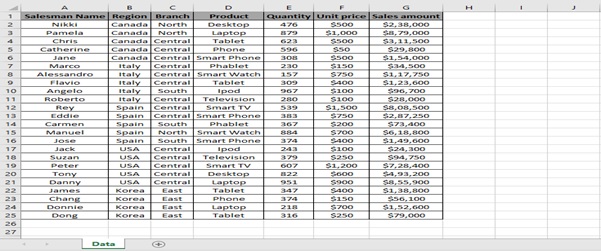
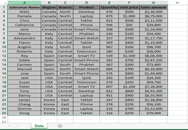
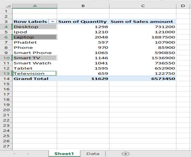
Let’s take an example of Sales information which looks as below.
We want to summarize sales amount by Screen size by grouping products by Large Display, Small Display & Others.
Step 1: Select the Sales table from A1 to G25
Step 2: Go to INSERT Tab
Step 3: Click on Pivot Table

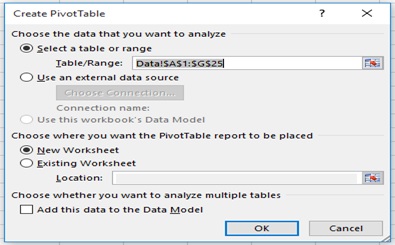
Step 4: Create PivotTable dialog box appears
Step 5: Click on OK
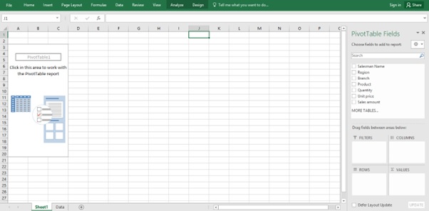
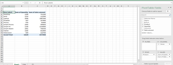
Step 6: Pivot Table fields appears in new sheet
Step 7: Drag Product to ROWS area
Step 8: Drag Quantity and Sales amount to VALUES area
Step 9: Now you start to group the Large Display products
Step 10: Select Desktop, Laptop, Smart TV & Television by press Ctrl key and selecting one by one.
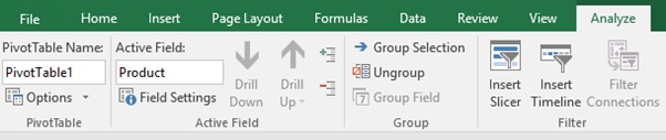
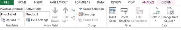
Step 11: Click on ANALYZE tab
Step 12: Click on à Group Selection option in the Group group

Step 13: You can see that Group1 is created
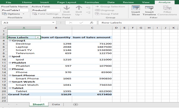
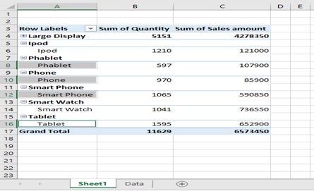
Step 14: Select the Group1 Cell A4 and change the name to “Large Display”in Formula bar
Step 15: Select Phablet, Phone, Smart Phone & Tabletby press Ctrl key and selecting one by one for creating Small Display group.
Step 16: Click on ANALYZE tab
Step 17: Click on à Group Selection option in the Group group

Step 18: You can see that Group2 is created
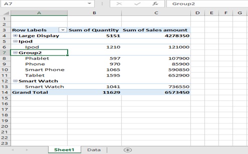
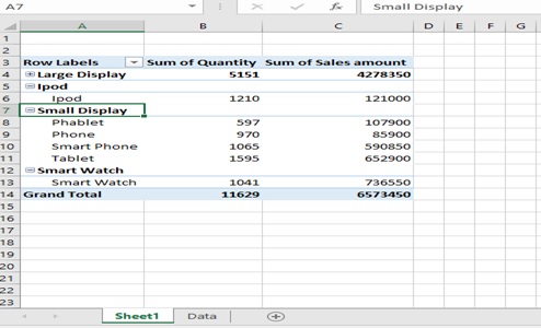
Step 19: Select the Group2 Cell A7 and change the name to “Small Display” in Formula bar
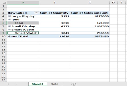
Step 20: Select Ipod and Smart Watch by press Ctrl key and selecting one by one for creating Others group
Step 21: Click on ANALYZE tab
Step 22: Click on à Group Selection option in the “Group” group
Step 23: You can see that Group3 is created
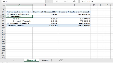
Step 24: Select the Group3 Cell A5 and change the name to “Others” in Formula bar
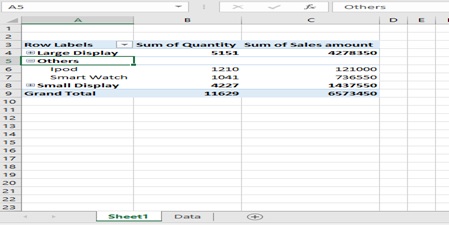
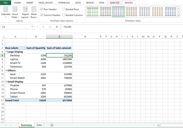
Step 25: Result of grouping
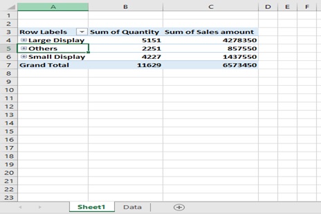
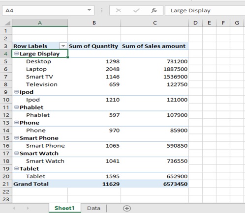
Step 26: Go to DESIGN tab
Step 27: Click on Show in Compact Form from Report Layout in Layout group
Note: You can Ungroup by selecting the Group name cell (Large Display, Small Display and Others) and select Ungroup from “Group” group in ANALYZE tab
Scope of Usage
- Can be used to select your options and place them under a group
- Can be used to create your own customized groups in a Pivot table
- Can be used to ungroup the groups which have been created